How to evaluate results
CENOS platform incorporates a powerfull post-processing tool - ParaView. It is being used all around the world by specialists of different fields ranging from Structural Analysis to CFD and Climate Research.
Being one of the most powerfull open source data analysis and visualization software, it has become complex enough to confuse new users about how to use it.
In this article we will look into some of the most common ParaView filters and their usage, as well as filters especially usefull in induction heating simulation result analysis.
How to choose which result values to compute
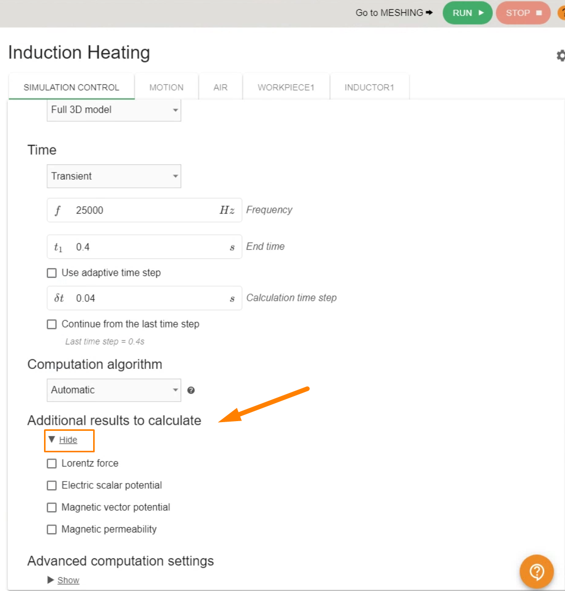
Before we dive into ParaView and its workings, we need to first understand what is being visualized in ParaView. By default ParaView shows us the visual result components, such as Temperature or Current Density, but you can add some aditional results, such as Lorentz Force, Electric scalar potential, Magnetic vector potential and magnetic permeability.
To add this results you should go to the Physics block and click on Show under the tab Aditional results to calculate
In there you can select or deselect values you want to calculate:
If you have calculated the case, but forgot to select a specific value, you can select it even after the calculation and recalculate only the result part to get the value of interest. Simply click Re-calculate to calculate the missing result values:
How to access filters
ParaView filters are algorithms that extracts a specific information such as iso-contours and point data from the initial result data set and are used to visualize specific physical properties of the calculated simulation.
Filters are accessible in different ways. If you know which filter you need, you can click Filters → Search... and search directly for the filter by entering its name in the Search window and clicking Enter.
In the example below the word plot has been written in the Search window, and all filters which names include plot are found and available for selection.

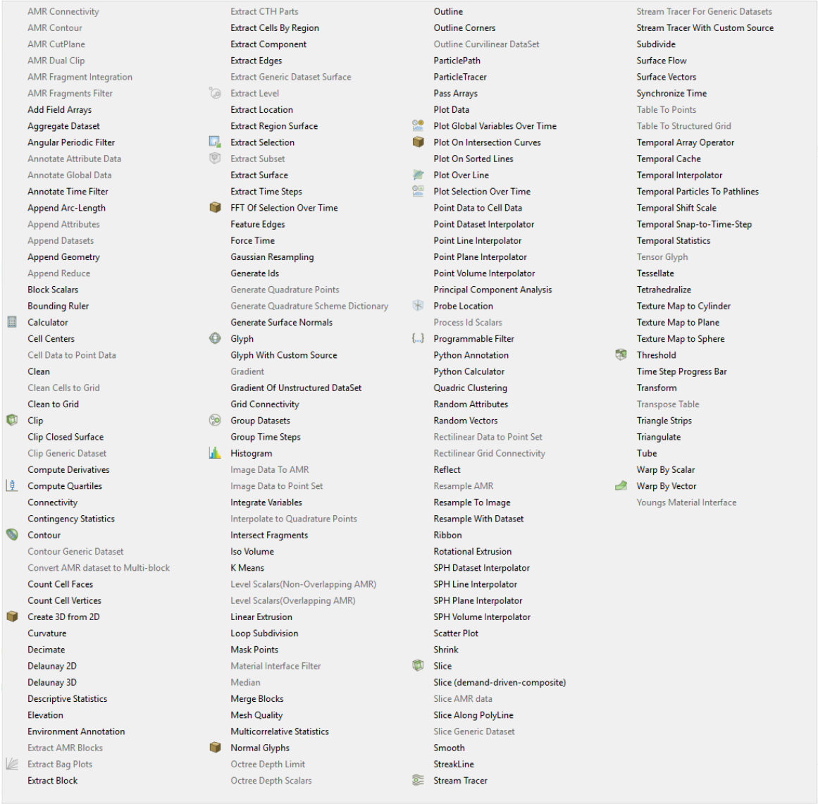
If you don't know which filter to use, you can choose from all filters available by clicking Filters → Alphabetical
How to use filters
In order to use ParaView filters, first a data set must be chosen on which the filter will apply. After the end of the calculation CENOS will open ParaView window with a pre-set state consisting of 1 result window (in 3D case) or 2 result windows (in axial symmetric 2D case). The simulation data will also be divided into smaller data sets, such as Workpiece, Inductor etc.
IMPORTANT: If you want to apply filters to a specific data set, you need to first select them from the Pipeline Browser.
For example, if you want to apply a filter such as Plot Over Line to the workpiece, the corresponding data set must be chosen before selecting the filter, otherwise none of the filters will be selectable.

Most commonly used filters
Filters that are most commonly used as the means of visual result evaluation are also the first ones to be used in order to determine the validity of the results. Even though they are not as complex as other filters, they are still important for the post-processing.
Extract Block
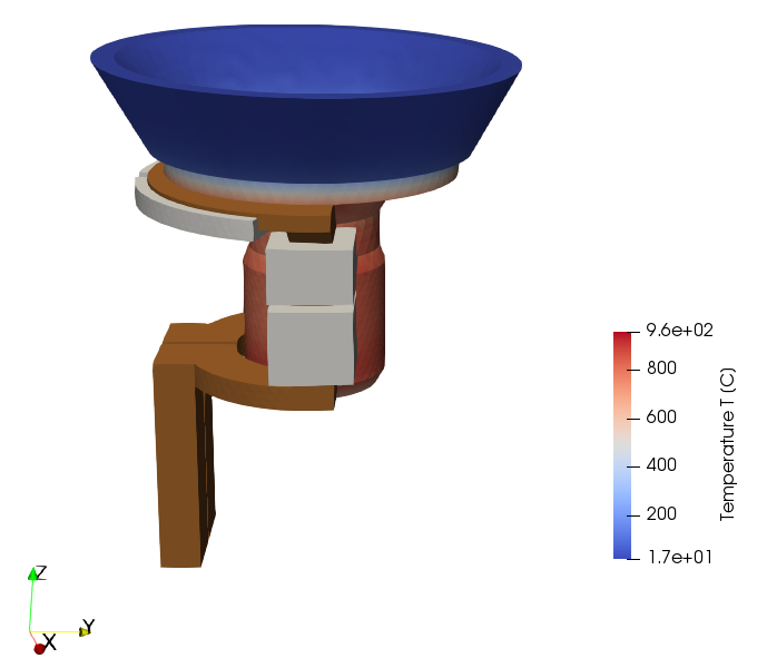
Extract Block allows to extract single or multiple domains from the full data set and manipulate the results in these domains independently. CENOS automatically exports data sets of workpiece and inductor domains, but Extract Block can be used even further.
For example, in single shot case CENOS automatically exports and visualizes the temperature distribution in the workpiece as well as a solid inductor.
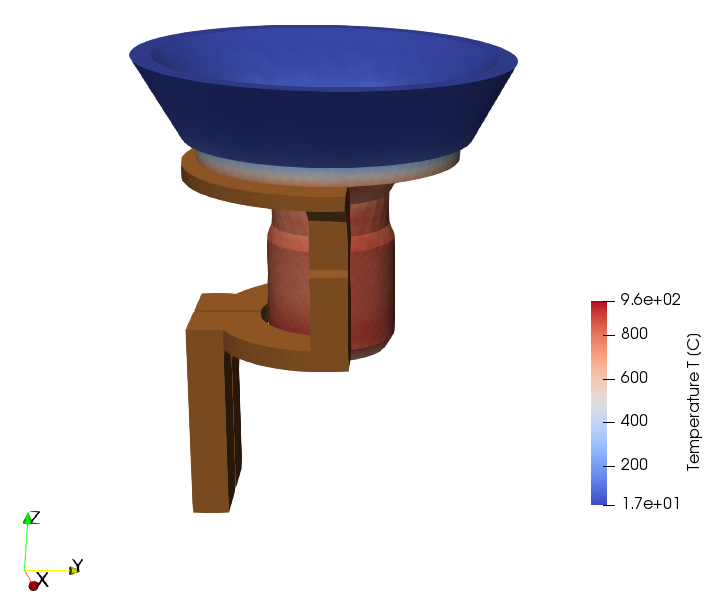
IMPORTANT: Because workpiece and inductor data sets have been exported seperately, we can manipulate results independently for each domain.
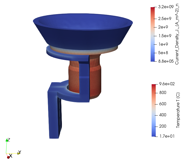
If we select Inductor from Pipeline Browser and change the visualization from Solid Color to Current Density, we can visualize the current flow in the inductor, while keeping the temperature distribution in the workpiece.
The single shot simulation incorporates concentrators around the coil, but they are not automatically exported. To visualize concentrators, select Simulation Data from Pipeline Browser and open Extract Block filter. In Properties window select concentrator domain (yoke in this case) and click Apply.
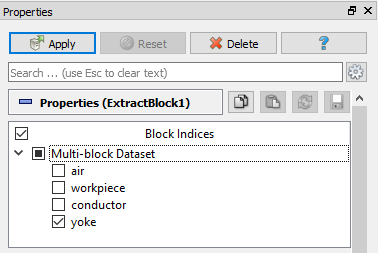
Select newly created ExtractBlock1 and change the visualization from Current Density to Solid Color.
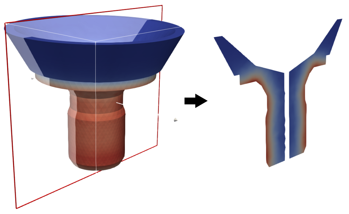
Slice
Slice allows to cut the domain with a plane and visualize only a layer of it.
To use Slice, select the domain of interest (extracted part or full computational domain) and open Slice filter. Under Properties enter the parameters that define the plane which will be used to create the slice.
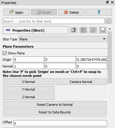
Uncheck the Show Plane box to turn off the visibility of the slice plane, and click Apply. Select Slice1 from Pipeline Browser and change the default Current Density visualization to Temperature.
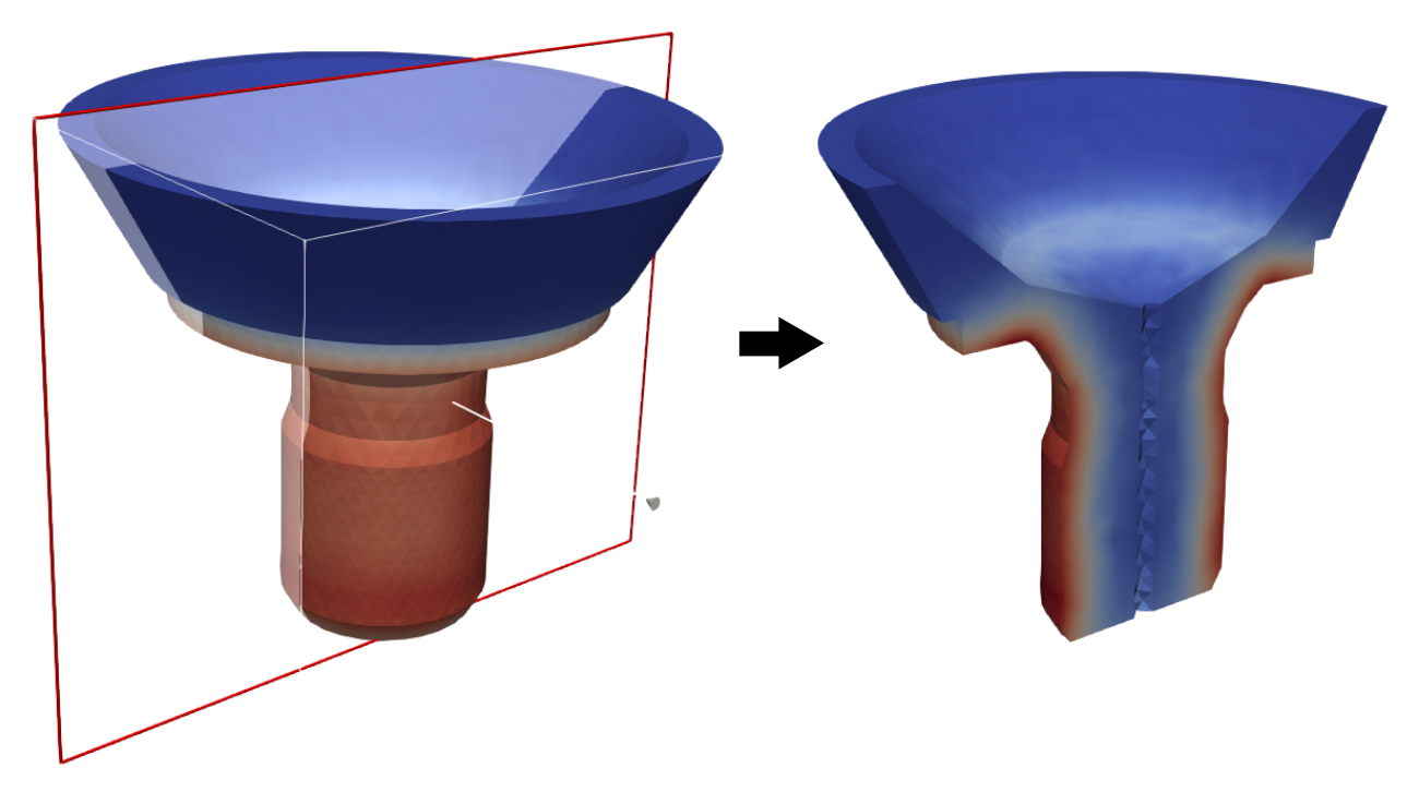
Clip
Clip is similar to the Slice filter and allows to cut the domain in half and visualize only a part of it.
To use Clip, select the domain of interest (extracted part or full computational domain) and open Clip filter. Under Properties enter the parameters that define the plane which will be used to create the clip.
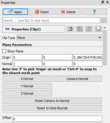
Uncheck the Show Plane box to turn off the visibility of the slice plane, and click Apply. Select Clip1 from Pipeline Browser and change the default Current Density visualization to Temperature.
Stream Tracer
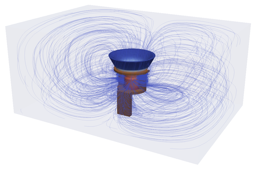
Stream Tracer allows to generate streamlines for vector fields. It is usefull for visualization of magnetic field lines.
In order to better visualize magnetic field lines, filter should be applied to the whole computational domain, because it generates streamlines within the selected domain, meaning that if you want to visualize magnetic field lines around your geometry, you need to generate streamlines in the air domain which encloses the geometry, not in the geometry itself.
IMPORTANT: To generate streamlines around the geometry, apply Stream Tracer to the air domain or to the whole computational domain, which contains the geometry.
To use Stream Tracer, select the domain of interest (select Simulation data for the whole computational domain), open Stream Tracer filter and click Apply.
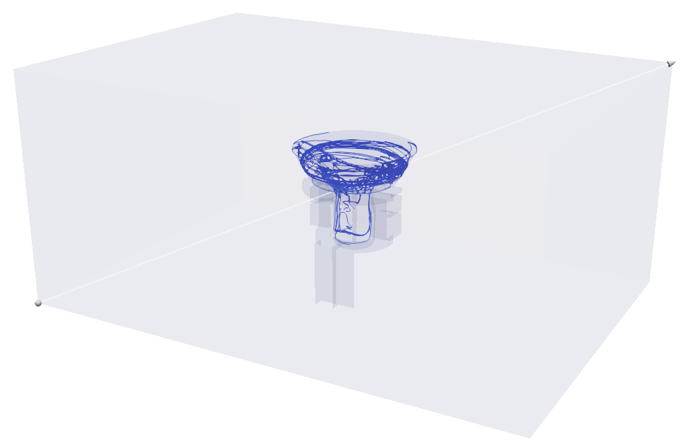
To better visualize magnetic field lines, change Vectors to Magnetic Flux Density, increase the Maximum Streamline Lenght, change Seed Type to Point Cloud, increase the sphere radius and Number Of Points, and decrease the Opacity.
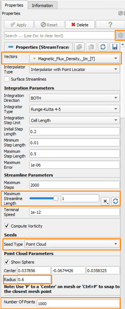
Extract and make visible the geometry you want to generate streamlines around, and with Stream Tracer properties adjusted, click Apply.
Filters useful for induction heating
Some filters and result evaluation methods are especially usefull for in-depth result analysis of induction heating simulations.
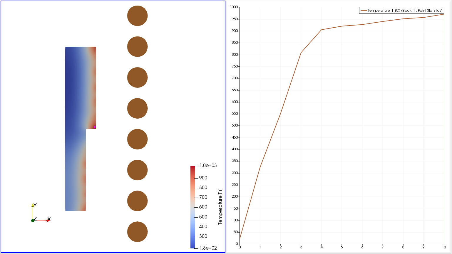
Plot Selection Over Time
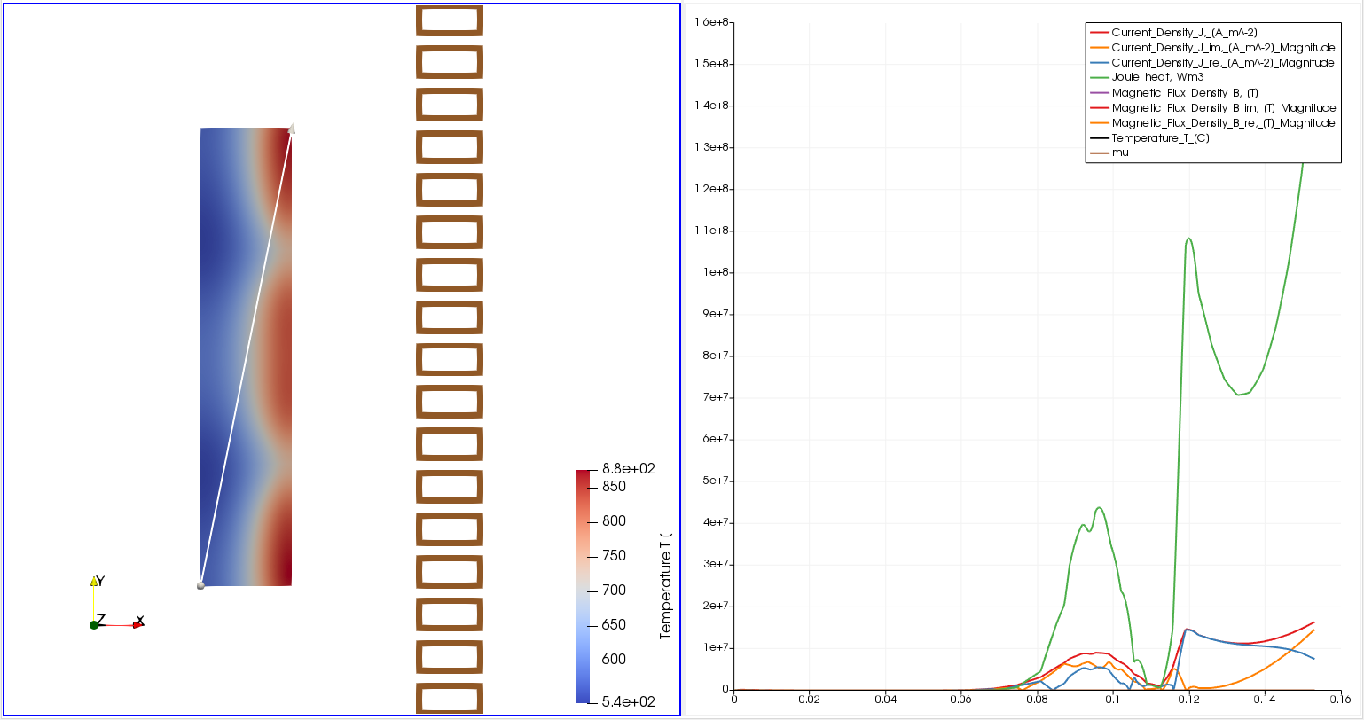
Plot Selection Over time enables you to plot time dependent graphs at a specified point.
To use Plot Selection Over time, first you need to mark your point of interest. Do that by clicking the "d" key on your keyboard and then left-click on your workpiece to mark the specified point.
IMPORTANT: You can plot graphs only at points where the mesh lines are intersecting.
To better understand which points are available for plotting, change the visual representation of the domain of interest from Surface to Surface With Edges, and select the point you want to plot a graph at.
When you have selected the point, select the domain of interest (extracted part or full computational domain), open Plot Selection Over Time filter and click Apply.
All available results will be plotted right next to your simulation results as time-dependent values.
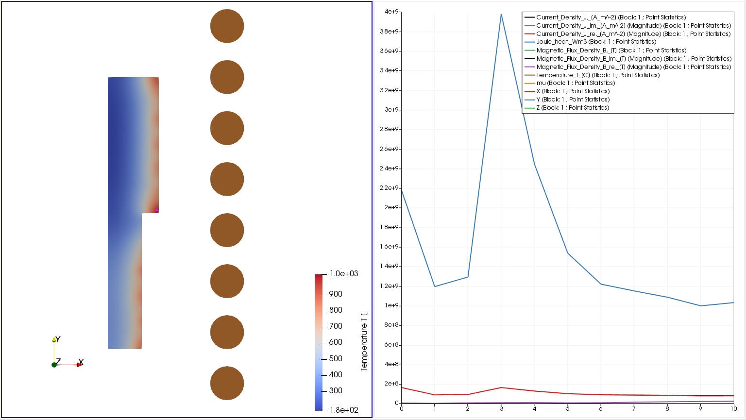
To switch between different results or plot a specific graph, select the window with graphs and in PlotSelectionOverTime1 Properties window under Series Parameters select only the Variables such as Temperature and click Apply to plot the new time dependent graph.
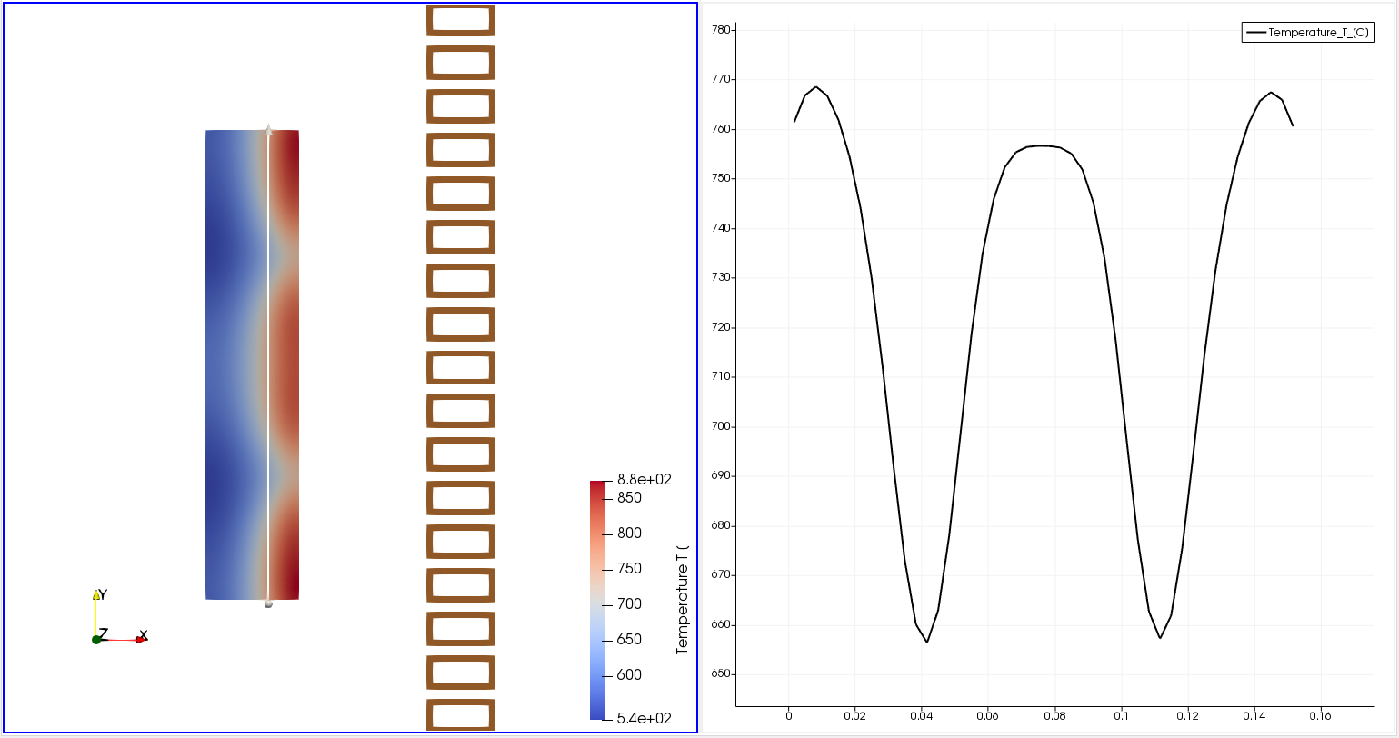
Plot Over Line
Plot Over Line allows to plot results along line drawn across the computational domain.
To use Plot Over Line, select the domain of interest (extracted part or full computational domain), open Plot Over Line filter and click Apply.
To switch between different results, select the window with graphs and in PlotOverLine1 Properties window under Series Parameters select only the Variables such as Temperature and click Apply to plot the new time graph.
IMPORTANT: You can adjust the line used to plot the graph by moving its starting and end point.
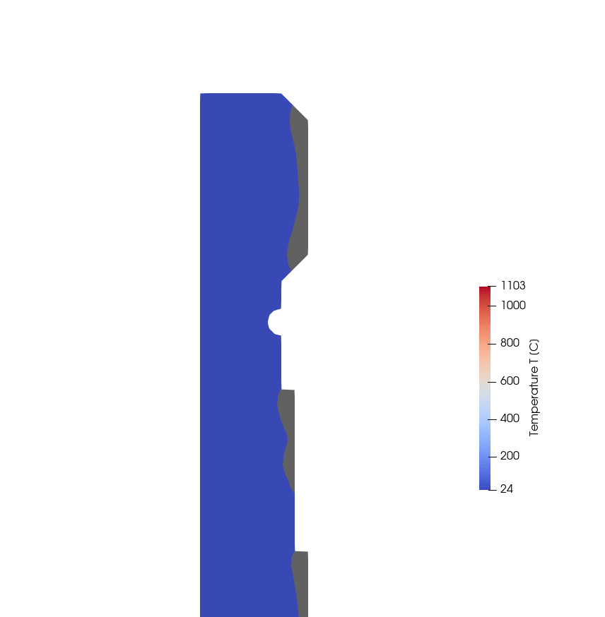
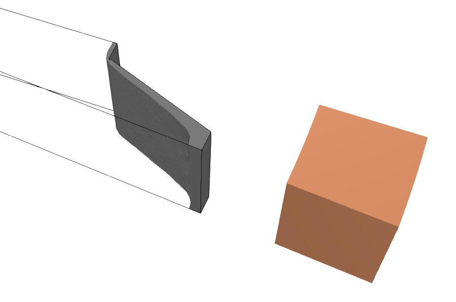
Hardened Zone
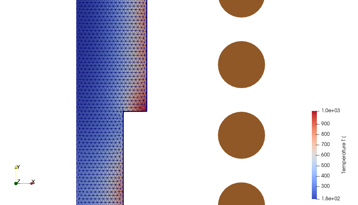
You can visualize the hardened zone with Hardened Profile filter. It creates a seperate zone in which the temperature at any time exceeds the austenization temperature.
To use Hardened Profile, select the domain of interest (workpiece), open Hardened Profile filter and click Apply.
IMPORTANT: In the Pipeline Browser click the Eye icon next to the workpiece to enable its visibility and see the hardened zone.
A seperate block in the pipeline browser will be created. You can change its color in the properties tab on the left with Edit color.

End result:
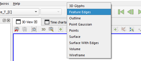
For 3D cases, once you have re-enable workpiece visibility, we suggest changing its representation mode (at the top) to Feature Edges:
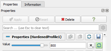
IMPORTANT: The default austenization temperature is 800 degC - find out and change the hardening temperature depending on your material!
Change the austenization temperature in HardenedProfile1 Properties window under Value Range.
Time charts
Once you have opened ParaView there will be two layouts created, 3D View and Time charts. This second layout contains various parameters from the .csv file plotted over time which show how Power, Voltage or any other parameter changes over time
![]()
After switching to the chart view, you will see four default charts showing various parameters. You can create custom charts by editing Script in the properties
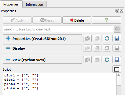
- Select the view by clicking anywhere in it
- Go to the Script window in the properties panel
- Enter the domain name in the first quotes
- Enter the parameter name from the .csv file in the second quotes
- Click anywhere in the chart view to refresh it
Example:
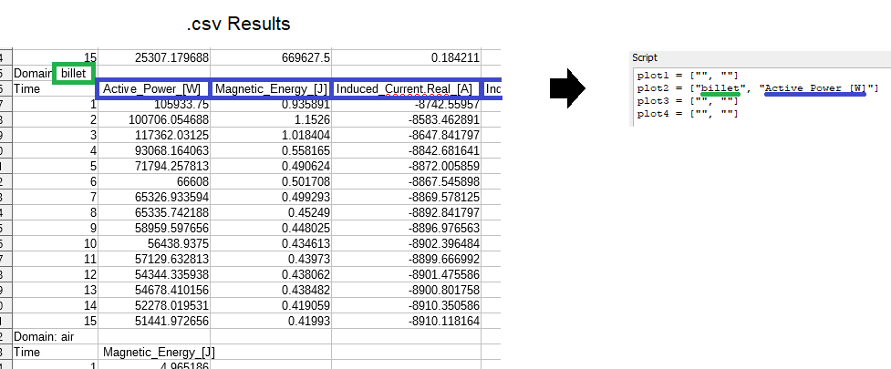
plot1 = ["", ""]
plot2 = ["billet", "ActivePower[W]"]
plot3 = ["", ""]
plot4 = ["", ""]
IMPORTANT: Make sure that there are no spaces in the begnning or end of the names, and that you have both quotes, otherwise the chart will not be drawn.